Machine Learning with Microsoft’s Azure ML — Credit Classification

Step-by-step model optimization for a highly imbalanced dataset using Azure ML

Microsoft’s Azure Machine Learning (AML) offers a host of productive experiences for building, training, and deploying machine learning models. At Clairvoyant, we employ AML for a wide range of use cases.

Banking on our experience of handling such challenges, this blog documents our step-by-step approach to model optimization in case of an imbalanced dataset using AML.
In this blog, we have used AML’s Python SDK (Software Development Kit), giving us greater flexibility to build and optimize models. We will be using a cleaned version of the German Credit Dataset for this exercise as sample data. Usually, credit classification data is highly disproportionate and skewed towards credible individuals. This disproportion leads to misclassification errors if not treated appropriately.

We will first explore the data well enough to help us formulate our approach towards model building and then use k-fold cross-validation and stratified sampling to tackle the problem of data imbalance. This approach can be extended to other similar datasets as well.

Before we start taking an initial peek at the data, let us briefly understand the project infrastructure. We will be using AML’s Python SDK with Jupyter Notebook for this experiment. The Python SDK gives much more freedom for model building than AML Designer and AML’s Automated ML service.

Microsoft Azure offers a host of popular services free of charge for 12 months and gives a $200 credit for the first 30 days. If you want to get some hands-on experience, the credit amount is more than sufficient for a month’s time.

The prerequisites to run models on AML are:

• Resource Group

• Workspace

• Compute

• Azure Machine Learning SDK

The setup instructions for the first three are here, and for Azure Machine Learning SDK refer to this link. You can find the entire documentation here.

Using Microsoft Azure Machine Learning for Model Training:

Once we have a resource group, a workspace and the compute instance, we connect to the workspace using AML SDK as follows:

import azureml.core

from azureml.core import Workspace

# Load the workspace from the saved config file

ws = Workspace.from_config()

print('Ready to use Azure ML {} to work with 
{}'.format(azureml.core.VERSION, ws.name))

Note: If you do not have a current authenticated session with your Azure subscription, you’ll be prompted to authenticate.

Azure ML allows users to

• Create logs that can be analyzed at a later instance

• Run python scripts using an estimator

• Create widgets to view information of every run

• Register a model for later use

• Register Datasets for later use

And much more. One can even create versions of their models as well as datasets and save them. We will be using the features mentioned above while simultaneously understanding our dataset and the modeling approach.

After establishing a connection to the workspace, we set up a run context for our experiment. In AML, an experiment can be thought of as a package consisting of :

• A dataset

• Modules connected to the dataset can be data transformations and models or both

from azureml.core import Run 

run = Run.get_context()

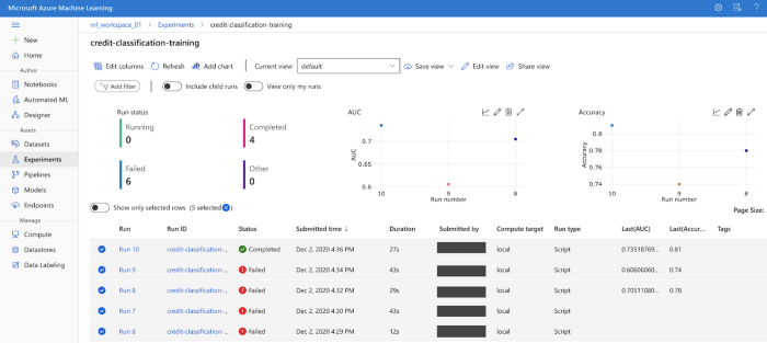
The console shows our experiment name as credit-classification-training, and we can see that several runs, both failed and completed, are tracked.

Understanding the Dataset:

Retail Credit classification categorizes individual borrowers based on their creditworthiness, calculated by considering several parameters. The dataset has several variables tracked for 1000 loan applicants and a target column (Credit_Classification) states whether an applicant is considered good or bad credit.

This is a supervised learning problem for binary classification, where 1 indicates bad credit and 0 indicates good credit. Some of the features are checking_account_Status, Credit_history, Purpose, Gender, Age, Foriegn_worker, etc.

We will see how these factors aid in extrapolating an individual’s creditworthiness.

Exploratory Data Analysis — EDA:

A first look shows us that the data is clean and has no null values in any features. As discussed in the beginning, we expect the data to be imbalanced and skewed towards credible individuals; you’ll find more 1s than 0s in the target column. This may feel intuitive as a financial institution usually has fewer defaulters than healthy accounts. Due to this disproportion, we do not perform outlier detection. If anything, there might be important information in the outliers that may help us identify bad credit.

AML allows us to save our images from a run and track them under the logging section. This helps preserve our research during EDA and comes in handy if we need to go back and take a look.

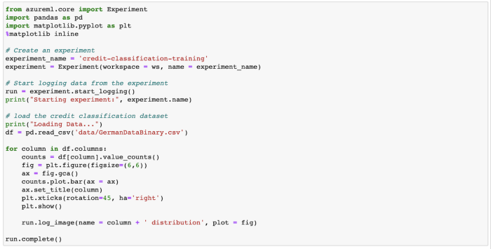
The code above looks at column distributions of the dataset. The plots created in matplotlib will be saved in the console as PNG files. The console looks as follows:

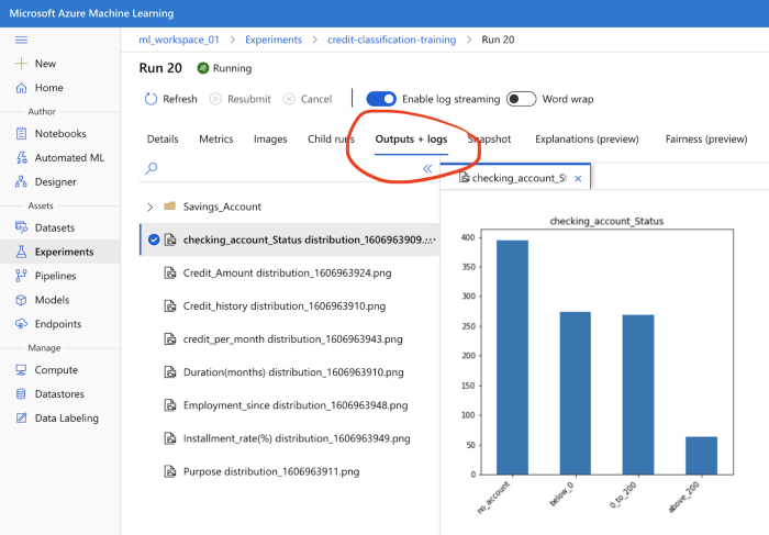
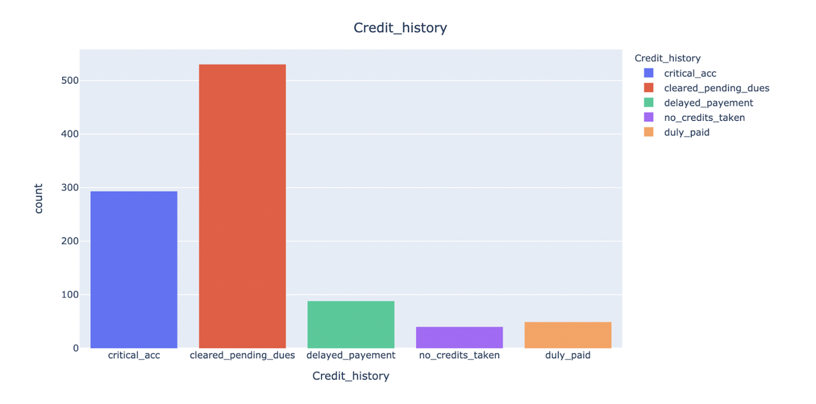
A deeper look into the internal structure of the data gives us an insight into a few patterns. From the following histograms, we can see that most of our applicants do not have a checking account.

Most of them have cleared their pending dues, although we have a substantial number of critical accounts too.

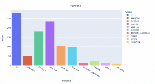
We can see that most of the applicants require financing for consumer durable products, such as consumer electronics, household furniture, etc. Further, finance required for used and new cars forms a significant chunk of the loan applications.

Similarly, by looking at other column distributions, we can say that unemployed individuals, individuals who do not own houses, married individuals, and a considerable female population do not apply for loans. Most of the loan applicants lack a guarantor or a co-applicant. Many loan applicants are skilled employees and more than 90% are foreign workers.

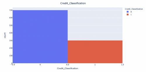
Finally, we can see the target column, Credit_Classification. There is a skewed distribution towards creditworthy customers. This confirms our expectation that applicants at risk of delinquency form a minority.

From the above observation, we can conclude that:

• there are two categories in the target variable, hence, binary classification

• the dataset is highly unbalanced

• this is a supervised learning problem and we use the column ‘Credit_Classification’ as our target variable

We can now move to pre-processing the data before we can push it into a machine learning model.

Feature Encoding:

Our dataset has several categorical variables, such as ‘Purpose’, ‘Employment_since’, etc. When we perform machine learning operations, we frequently come across categorical variables, but machines cannot comprehend strings. The categories need to be encoded into numerical values.

In our data, there are some nominal features and some ordinal features. We encode both of these separately. We perform one-hot encoding for nominal features using the pandas get_dummies function, whereas the ordinal features are encoded using sklearns, OrdinalEncoder.

Data Splitting:

We first split our data into features and target variables. In our case, the target variable is ‘Credit_Classification’ and all the other columns form our feature set.

Next, we perform a train-test split. We use sklearn’s train_test_split module to divide the dataset.

Training and Evaluation:

We now walk through model building, optimization, and interpretation of the Random Forest Classifier. Random Forest is a machine learning model used both for regression and classification. It is an ensemble of N small decision trees, where N is a large number. Prediction of each of these trees is combined together to form a robust and accurate forecast.

In comparison to linear models, Random Forest is more complex and hence interpretability takes a hit. These models also require high compute and take longer to build. But since it is robust and gives good results for classification, it is used extensively by data scientists.

To interpret model performance, we will be using two critical metrics for classification- accuracy and AUC ROC score.

We will employ a step-by-step optimization of the model. We will start with a base model and improve it using hyper-parameter tuning. Next, we will use cross-validation, and finally we will add to it stratified sampling.

Step 1: Base Model

Random state is used to seed the random number generator to ensure that the random numbers are generated in the same order. Our basic model is the Random Forest classifier with default parameters. We only set the random_state to 20 to reproduce the results.

from sklearn.ensemble import RandomForestClassifier 

classifier = RandomForestClassifier(random_state=20)

model = classifier.fit(x_train, y_train) 

prediction = model.predict(X_test)

The performance metrics of this model are shown below:

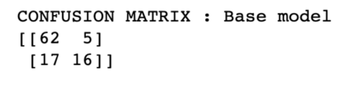
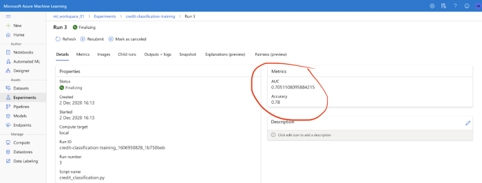
The confusion matrix here shows skewed results, which is expected as our dataset is highly imbalanced. The AML console shows that the accuracy score is 78% and the AUC-ROC score is 0.71. We will see if we can improve these numbers by tuning the model.

Step 2: Tuned Model

Every model takes in parameters, and every parameter takes in a range of values. When these parameters are fed to the model, it forms many permutations. Manually running one model for every permutation is infeasible. This is where sklearn’s RandomizedSearchCV module helps.

RandomizedSearchCV is used to tune parameters for a model automatically. It randomly selects parameter combinations, unlike the GridSearchCV, which uses every combination.

We define the parameter values in a dictionary and pass it to RandomForestClassifier(). In the end, this gives us the best parameters based on our scoring criterion. Since this is a classification problem, our scoring criterion is ‘roc_auc’.

from sklearn.model_selection import RandomizedSearchCV 
  
classifier = RandomForestClassifier() 
  
params = { 
  
‘n_estimators’: [100, 300, 500, 800, 1200], 
  
‘max_depth’: [5, 8, 15, 25, 30], 
  
‘min_samples_split’: [2, 5, 10, 15, 100], 
  
‘min_samples_leaf’: [1, 2, 5, 10], 
  
‘random_state’: [0, 10, 20, 50, 100, 200], 
  
}
  
random_search = RandomizedSearchCV(classifier, 

param_distributions=params, n_iter=5, scoring=’roc_auc’)
  
best_model = random_search.fit(x_train, y_train) 
  
print(best_model.best_estimator_.get_params())

Azure ML allows us to load our python script and pass in environment variables as parameters to an estimator. The code for that is as follows.

from azureml.train.estimator import Estimator 
  
from azureml.core import Experiment 
  
# Create an estimator 
  
estimator = Estimator(source_directory=training_folder, 
  
entry_script=’credit_classification_tuned.py’, 
  
compute_target=’local’, 
  
conda_packages=[‘scikit-learn’]) 
  
# Create an experiment 
  
experiment_name = ‘credit-classification-training’ 
  
experiment = Experiment(workspace = ws, name = experiment_name) 
  
# Run the experiment based on the estimator 
  
run = experiment.submit(config=estimator) 
  
run.wait_for_completion(show_output=True)

Following are the model metrics tracked via Azure ML.

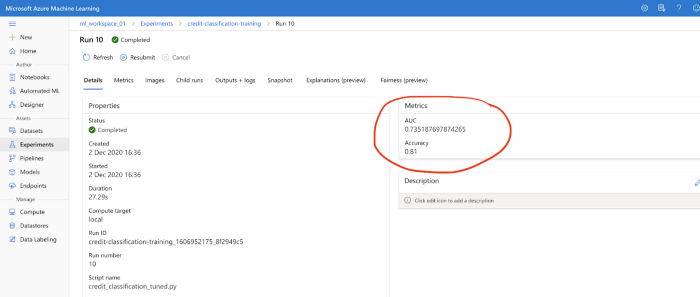
It is evident from the performance metrics that the auc_roc_score and accuracy have slightly increased.

Step 3: K-fold Cross-Validation

Cross-validation is a model validation technique which is sometimes called rotation sampling or out of sample testing. This technique is especially used when data is limited. It has a single parameter k, which is the number of partitions we want to divide the data into.

It works as follows- Say we have 1000 records and the value of k=10, then the data is divided into 10 parts, and 10 models are run over it. The first model trains parts 1 through 9 and tests on part 10. The second model trains on parts 1, 3 until 10, and tests on part 2 and so on.

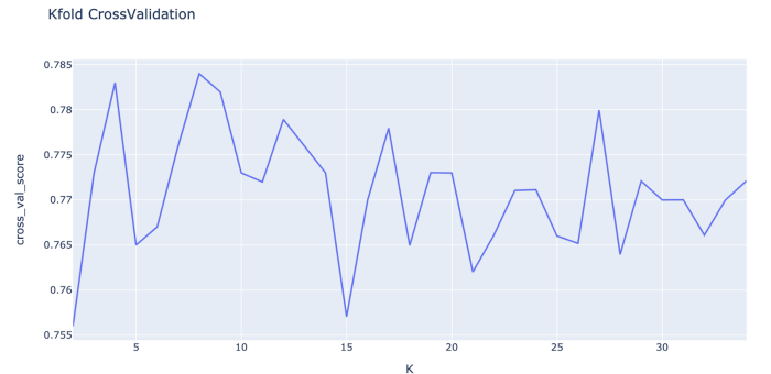
For our credit classification dataset, we want to choose the best value of k. Hence we plot the score for each k from 2 to 35 and choose k with the max score.

Clearly, the highest score is for k=8. With this value of k the best model accuracy is 85.58% and the lower end is at 71.76%

# Cross-validation for k = 8 
  
from sklearn.model_selection import cross_val_score score=cross_val_score
  
(classifier, X, y, scoring=”roc_auc”, cv=8)

Step 4: Stratified Cross-Validation

Finally, we deal with the problem that our data is imbalanced. Classifying bad credit correctly is more important than classifying good credit accurately. It generates more losses when a bad customer is tagged as a good customer than when a good customer is tagged as a bad one. The errors of misclassification are due to the skewed dataset and one solution to this problem is Stratified Cross-Validation.

In stratified k-fold cross-validation, the folds are made by preserving the percentage of samples for each class, unlike general k-fold cross-validation where samples are created randomly. This helps to eliminate sampling bias.

The following graph plots the cross-validation score over a range of values.

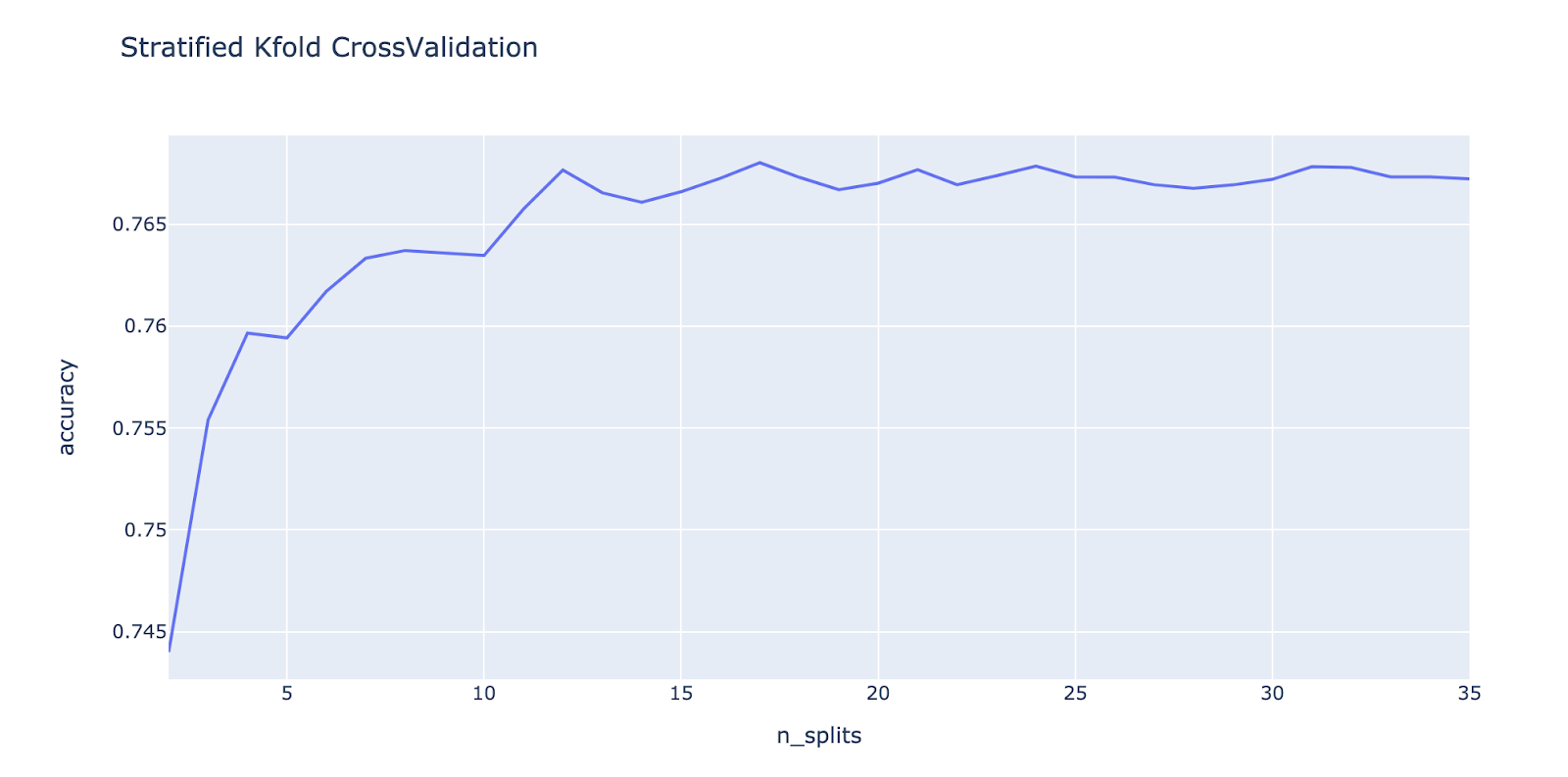
In the graph, even though the max accuracy is for n_splits = 17, by running for multiple values we can see that we get the best results for n_splits = 9. Here, we keep the random_state constant at 10.

The model accuracy ranges from 87.38% to 74.10%, which is a significant improvement.

Conclusion:

Our model optimization approach improved the accuracy of the model while moving step-by-step from the base model to the final model. Stratified sampling is an efficient method for imbalanced datasets, and we encourage you to use this stepwise guide and Azure Machine Learning to solve similar challenges.

We would also like to bring your attention to the project infrastructure. Azure machine learning makes it simple to use a robust environment, log experiment progress, track model and dataset versions, parametrize model building, and use compute resources on the go.

At Clairvoyant, we use Azure Machine Learning for a host of services in addition to the ones mentioned in this blog. AML is extremely flexible and provides an Enterprise-grade machine learning service to build and deploy models faster. For all your cloud based services requirements, contact us at Clairvoyant.

AML’s Python SDK gives more control to the user to build, register and deploy models and take advantage of the seamless Azure environment. In addition to the Python SDK, one can also use:

• Automated ML to build multiple models with a minimum amount of code

• Designer to drag and drop functionalities and create pipelines that can be used for inferencing and deploying, and a lot more. AML makes machine learning smooth, easy and fun!

  To learn about machine learning with Amazon SageMaker, read this blog.