4 Important and Effective Statistical Models to Forecast your Demand

We generally rely on historical data to help us predict the future. But how do these individual chunks of data become a projection of the future?

This blog will walk you through the basics of a few mathematical models that statisticians use when they are supposed to make sense out of these individual chunks of data. Let’s start by calling these individual chunks “Datasets”.

Clairvoyant has helped multiple businesses forecast and predict their future sales with statistical models. With Clairvoyant’s predictive analytics solutions, you will always be one step ahead of your competitor. Our solutions are future-ready and capable of altering the course of action depending upon the climatic, social, or governmental conditions at that period of time.

Let’s take a look at a few statistical models and see which one fits your unique business needs the best-

Deep Neural Network (DNN)

This predictive analytics technique is for you if:

• You are a new entrant in the market
• You are introducing a new product line
• You don’t have any historical data in place for the new product that you are looking to launch

Why is DNN the right model for you?

If you are a new entrant in the market looking to manufacture chocolates, it is safe to assume that you do not have any historical data to forecast the demand. With DNN, you can train the algorithm with the weekly sales data of a similar dataset (in this case, your competitor’s chocolate sales data) to estimate the demand for your SKU (Stock Keeping Unit). You can also add external data, such as data about the category, to increase the accuracy of the demand forecast.

How does DNN function?

Initially, the DNN model scans through several layers of networks to try and find a correct mathematical manipulation that converts the input into output (demand forecast). As it progresses, it carefully analyzes every layer to calculate each output’s probability.

The DNN model then examines the data of the lookalikes in place of the actual data, since the latter is not available. The ‘similar’ or ‘lookalike’ product’s price, features, attributes, etc. are taken into account to forecast the demand.

The DNN model is trained on the SKU data that you possess, and it will try to understand the relationship between the input and output variables. This gives you an idea of your desired output, enabling you to tune the model accordingly. In order to minimize errors, you can add more data to get accurate predictions.

Benefits of the DNN model

• The model considers a variety of data such as external, internal, numerical and categorical to increase the output accuracy
• It looks for and considers complex dependencies in both linear and non-linear data. This allows for increased accuracy in the output
• It comes handy when companies look to forecast demand among complex seasonalities

Limitations of the DNN model

• Unless a data scientist instructs the model not to consider a particular factor, the model will not comprehend the factor’s impact on the output.
• If a data scientist fails to train a DNN model well, it may not be able to differentiate between faulty and accurate data. The model may still produce accurate forecasts based on the training data but may generate erroneous output in the incoming data. This phenomenon is called overfitting.
• Untrained users and companies may perceive the model as a magic box that generates results out of nowhere. A statistician may need to explain its working to its users.

Example

Problem: Statisticians at the Blekinge Institute of Technology used DNN to forecast the volume of packaging material for Volvo Logistics AB’s vehicles for the upcoming year.

They observed that the packaging demand at the facility was influenced by several factors, such as product demand, lead times, regulatory requirements, packaging innovations, etc.

To train the model, the statisticians gathered the following data-

• 6 months’ transaction data of the packaging materials
• Historical vehicle production volume data
• Projected vehicle production volume data

A hybrid CNN-LSTM (Convolutional Neural Network- Long Short-Term Memory) model was chosen to generate the output. CNN and LSTM are also DNN models but a hybrid was chosen as it showed better results than their respective individual models.

Result

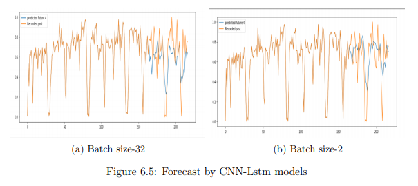
As CNN-LSTM models were able to learn the purchase patterns, they were able to forecast peak and low demands better than their respective individual models.

How to get an efficient DNN model tailored to your unique business needs?

Want a quick and perfect Deep Neural Network set up for your business? 

Here it is! Being a data analytics company, Clairvoyant can install the DNN model and train the algorithms to suit your business needs. The model is fine-tuned to generate accurate and error-free results.

Linear Regression (LR) 

This predictive analytics technique is for you if:

• You want to explore how different factors can impact your business
• You want to predict the impact of an independent variable on a dependent variable. For example, if you wish to predict the increase in sales of Air Conditioners (dependent variable) based on the increase in temperature (an independent variable), you can use the Linear regression model

Why is LR the right model for you?

We all may have faced a situation like this- the demand for your good suddenly goes up post a successful marketing campaign, but you do not have enough stock to fulfill that demand. Linear regression comes handy when you know that your demand will increase or decrease based on certain independent variables. Applying the same example given above, if the temperature of a certain city increases during the summer, the sales of AC goes up too. On the contrary, as the temperature starts decreasing, the sales numbers decrease too. This example is the simplest way of demonstrating how independent variables affect the dependent variable. You can look at the following situations where using LR could be the right choice-

• You are aware of all the independent variables that affect your dependent variables
• None of these independent variables are dependent on each other
• You are aware of a possible one-to-one variation that can be established between the dependent and independent variables

How does LR function?

The straight-line equation, y = mx + c, is the simplest explanation of how LR works.

In the equation,

y = dependent variable,

x = independent variable,

m = slope of the line, and

c = the y-intercept (value of y when x=0)

LR’s core intention is to obtain a line that best fits the data. The line with the smallest total prediction error is the best-fit line. The error is the distance between the point to the regression line. This function could be extrapolated with multiple independent variables too.

y=mx+nz+ow+c where x,z,w are independent variables and have no correlation between them. m,n,o are slope by which each of these variables impacts the dependent variable.

Example

Problem: An investor wants to invest in a growing start-up and wants to determine if the investment will be profitable in 2021. So, instead of investing a ton of money, he decides to buy a few shares. And for this example, let’s consider that these stock prices are dependent on the sales of the start-up.

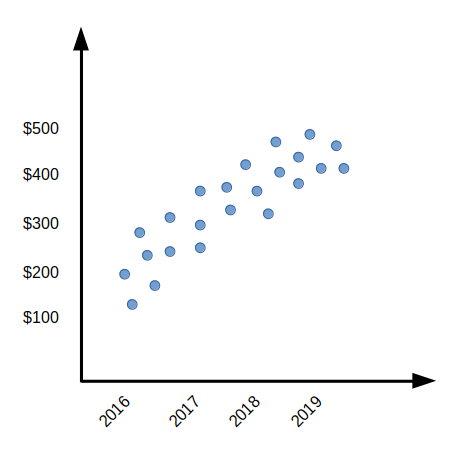
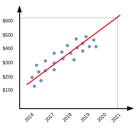
The scatter plot above shows a trend in stock prices. The prices have grown from $100 to $500 with the sales reaching 1 billion from 200 Million. Examining the trend in the graph, it is safe to assume that the company might grow further and not encounter a drastic fall. The LR model can help the investor predict the stock prices’ growth over the projected period.

Benefits of the LR model

• It’s simple and efficient!
• Only when trained on large datasets can it generate faster outputs

Limitations of the LR model

• It functions better on linear data than on non-linear data. It is necessary to determine if the data variable is linear. Linear aggression, which has linear in its name, can be used only when the user deals with linear variables that graphically represent a straight line
• Linear regression can only be carried out in a case that tends to be more frequent, such as sales

Time Series Forecasting (TSF)

This predictive analytics technique is for you if:

• you are the owner of a majorly seasonal business (eg — Tourism, Hotel, Clothing, etc.)
• Individuals who run their businesses based on trends, cycles, or irregularities

Why is Time series the right model for you?

As the model’s name suggests, Time-series analysis focuses on the ‘time’ component. If you want to understand the demand of your product during a particular period, time-series is the model for you.

Time plays a crucial role in the time-series model as its output depends on a particular time frame. It studies the historical data to predict when the wave from a past trend will hit back. Businesses that are cyclic in nature make use of time-series models to estimate their growth, recession, and recovery and when they might encounter one of them again. Time-series also aid the financial sector in projecting stock market analysis, economic forecast, yield projections, etc.

How does the Time-series model function?

• Make the data stationary- to make the data stationary in an ARIMA model Time-series forecast, remove any noise from the data. Remove the trend, seasons, correlation, and other such factors present in the data, so that the mean of the series is no longer a function of time. You can remove this ‘noise’ by calculating the difference between consecutive observations.
• Establish a base level forecast- In this step, you decide the appropriate base-level model for your time-series forecast depending on the type of data you possess. If your data has seasonal trends, an Exponential Smoothing Model (ESM) would be an ideal base-level model choice for you. This model gives the maximum weightage to the most recent value in the data while assigning the least weightage to the ones before.
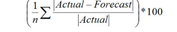
• The final step would be to measure the model’s accuracy. Calculating MAPE (Mean Absolute Percent Error) is an easy way of doing this. Below is the formula for MAPE

Benefits of TSF model

• The statistical technique has been developed in such a way that the factor that influences the fluctuation of the series may be identified during the process of forecasting the demand
• It helps to compare the performance of two different series during the same time duration
• The analysis by time-series helps us compare the present performance of the series against its past

Limitations of the TSF model

• Time series analysis cannot fully adjust to a variety of factors that may affect the fluctuations of the series
• The factors on which the time series analysis is performed may not remain constant for a long time and hence the predictions made using them may be unreliable in the longer run
• It becomes difficult to understand the trend unless modifications are made to the database, as sometimes, factors like the increase in the human population might be a reason for the increasing trend in the time series

Example

Problem — A retail company wants to calculate and forecast its summer sales for the year 2003.

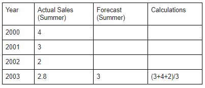
To find the accurate numeric output, the company has used the Moving-Average method under Time-Series. For this calculation, the Actual Sales of the previous years are added and then divided by the number of years.

(3+4+2)/3 = 3

So the forecasted sales for the year 2003 is 3 and the actual sales is 2.8

Moving average method is commonly used in the retail industry as it eliminates the noise in the product's pricing structure for a given time.

Classification And Regression Trees (CART)

This predictive analytics technique is for you if:

You cannot achieve a linear or nonlinear linking function between your dependent and independent variables but are sure that the independent variable affects the dependent variable. CART removes the assumption that the dependent and independent variables are monotonic. Instead, it creates a decision tree where predictions are made based on multiple recursive binary splits.

Why is CART the right model for you?

One of the preconditions of using a classification model is that your dependent variable can take only one of two mutually exclusive values at a time. Because these responses are binary, it is impossible to find a linear, or linking relationship between the dependent and independent variables. Hence you should use the classification tree method when you are trying to predict a variable that generally has binary mutually exclusive responses.

How does CART function?

A CART function generally divides the entire prediction process into multiple steps; we can refer to each one of them as feature splits. In each of these splits, a binary decision is taken to decide whether the value should be predicted or should the system be directed to another split (explained in the diagram above). The question on how to decide the feature splits could be answered using three variables; entropy of your data set, information gain of your data set, and Gini index of your dataset. You can read more about this here. But what these splits help you achieve is the capacity to drill down the prediction of a variable into a binary decision-making process and not dependent on a linking function as with linear or logistic regression.

Benefits of the CART model

• The CART algorithm is a machine algorithm that can improve itself to improve information gain at every point.
• The model allows its users to read and interpret both numerical and categorical data
• The performance of the decision trees are not affected by the relationship of non-linear trees

Limitations of the CART model

• There is a small possibility that the tree may not come up with accurate results if there is a lot of noise present in the data
• The stability of the data can be affected even by a small variance (in the data) as it may lead to high variance in the model’s predictions
• Sometimes a complex decision tree may have a low bias, making it difficult to incorporate new data into the model

Conclusion

A variety of statistical techniques can be used to predict or forecast future demands or otherwise unknown events. Statistical techniques also forecast customers' buying behaviour and influence variables, such as time, patterns (sales), inventory forecasting, risk forecasting, etc. 

Each statistical model is unique in nature and has a different application. Depending on the need and nature of your business, a unique statistical model can be used to drive predictions for accurate results. 

Check out our artificial intelligence services for all your business requirements.