A Brief on the Key Information Measures used in a Decision Tree Algorithm
The decision tree algorithm is one of the widely used methods for inductive inference. Decision tree approximates discrete-valued target functions while being robust to noisy data and learns complex patterns in the data. In the past, we have dealt with similar noisy data; you can check the case studies that revolve around this here.
The family of decision tree learning algorithms includes algorithms like ID3, CART, ASSISTANT, etc. They have supervised learning algorithms used for both classification and regression tasks. They classify the instances by sorting down the decision tree from root to a leaf node that provides the classification of the instance. Each node in the decision tree represents a test of an attribute of the instance, and a branch descending from that node indicates one of the possible values for that attribute. So, classification of an instance starts at a root node of the decision tree, tests an attribute at this node, then moves down the tree branch corresponding to the value of the attribute. This process is then repeated for the subtree rooted at the new node.
The main idea of a decision tree algorithm is to identify the features that contain the most information regarding the target feature and then split the dataset along the values of these features. The target feature values at the resulting nodes are as pure as possible. A feature that best separates the uncertainty from information about the target feature is said to be the most informative feature. The search process for the most informative feature goes on until we end up with pure leaf nodes.
The process of building an Artificial Intelligence decision tree model involves asking a question at every instance and then continuing with the split - When there are multiple features that decide the target value of a particular instance, which feature should be chosen as the root node to start the splitting process? And in which order should we continue choosing the features at every further split at a node? Here comes the need to measure the informativeness of the features and use the feature with the most information as the feature on which the data is split. This informativeness is given by a measure called ‘information gain.’ And for this, we need to understand the entropy of the dataset.
Entropy
It is used to measure the impurity or randomness of a dataset. Imagine choosing a yellow ball from a box of just yellow balls (say 100 yellow balls). Then this box is displayed to have 0 entropy which implies 0 impurity or total purity.
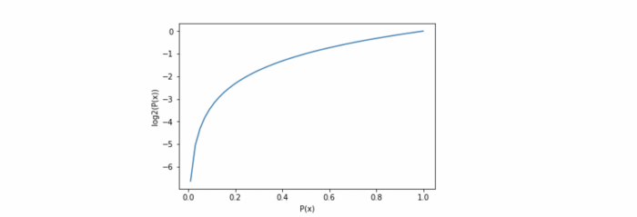
Now, let’s say 30 of these balls are replaced by red and 20 by blue. If we now draw another ball from the box, the probability of drawing a yellow ball will drop from 1.0 to 0.5. Since the impurity has increased, entropy has also increased while purity has decreased. Shannon’s entropy model uses the logarithm function with base 2 (log2(P(x)) to measure the entropy because as the probability P(x) of randomly drawing a yellow ball increases, the result approaches closer to binary logarithm 1, as shown in the graph below.
When a target feature contains more than one type of element (balls of different colors in a box), it is useful, to sum up the entropies of each possible target value and weigh it by the probability of getting these values assuming a random draw. This finally leads us to the formal definition of Shannon’s entropy which serves as the baseline for the information gain calculation:

Where P(x=k) is the probability that a target feature takes a specific value, k.
The logarithm of fractions gives a negative value, and hence a ‘-‘ sign is used in the entropy formula to negate these negative values. The maximum value for entropy depends on the number of classes.
- 2 Classes: Max entropy is 1
- 4 Classes: Max entropy is 2
- 8 Classes: Max entropy is 3
- 16 Classes: Max entropy is 4
Information Gain
To find the best feature that serves as a root node in terms of information gain, we first use each defining feature, split the dataset along the values of these descriptive features, and then calculate the entropy of the dataset. This gives us the remaining entropy once we have split the dataset along with the feature values. Then, we subtract this value from the initially calculated entropy of the dataset to see how much this feature splitting reduces the original entropy, which gives the information gain of a feature and is calculated as:

- The feature with the largest entropy information gain should be the root node to build the decision tree.
ID3 algorithm uses information gain for constructing the decision tree.
Gini Index
It is calculated by subtracting the sum of squared probabilities of each class from one. It favors larger partitions and is easy to implement, whereas information gain favors smaller partitions with distinct values.

A feature with a lower Gini index is chosen for a split.
The classic CART algorithm uses the Gini Index for constructing the decision tree.
Conclusion
Information is a measure of a reduction of uncertainty. It represents the expected amount of information that would be needed to place a new instance in a particular class. These informativeness measures form the base for any decision tree algorithms. When we use Information Gain that uses Entropy as the base calculation, we have a wider range of results, whereas the Gini Index caps at one.
Resources for further exploration:
Book — Machine learning by Tom M. Mitchell