Let’s understand Spark’s logical and physical plans in detail!
Clairvoyant aims to explore the core concepts of Apache Spark and other big data technologies to provide the best-optimized solutions to its clients. In light of the recent performance enhancements, we have utilized fundamental information about the query plans in Spark SQL and details about the query execution to achieve a more optimal plan to ensure efficient execution.
The objective of this blog is to document the understanding and familiarity of physical and logical plans in Spark, and use that knowledge to achieve better performance of Apache Spark. We will walk you through some relevant information that can be useful to understand a few details about the execution.
Thank you, Shubham Bhumkar(Co-Author/Contributor), for your valuable inputs in improving the quality and content of the blog.
What is Spark Logical Plan?
Logical Plan refers to an abstract of all transformation steps that need to be executed. However, it does not provide details about the Driver(Master Node) or Executor (Worker Node). The SparkContext is responsible for generating and storing it. This helps us to achieve the most optimized version from the user expression.
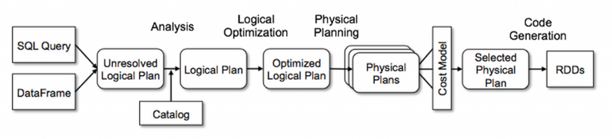 Flow Diagram For Query Plans
In layman's terms, a logical plan is a tree that represents both schema and data. These trees are manipulated and optimized by a catalyst framework.
The Logical Plan is divided into three parts:
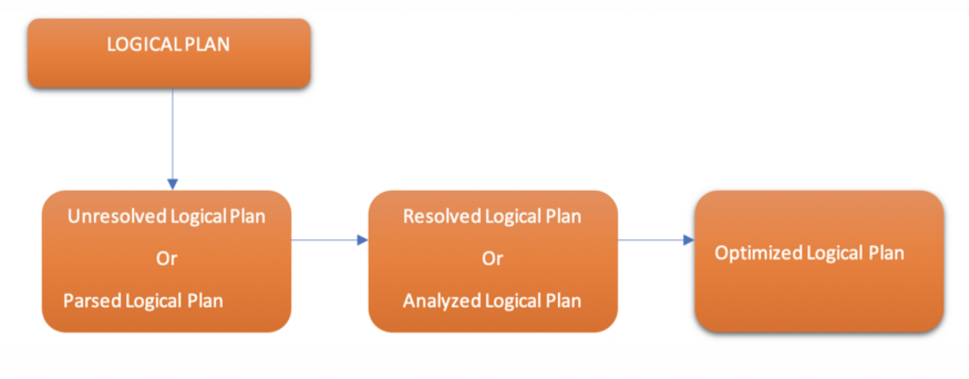 Logical Plan Sequential steps
We will first create an RDD of numbers ranging from 0 to 100 as shown below:
 RDD creation
We will be using the ‘explain’ command to see the plan of a DataFrame.
We should run the ‘explain’ command with a true argument to see both physical and logical plans. The physical plan is always an RDD. It gives only the physical plan if we run it without the true argument.
(i) When ‘explain’ command is used without the true argument:
 explain function without true argument
(ii) When ‘explain’ is used with the true argument:
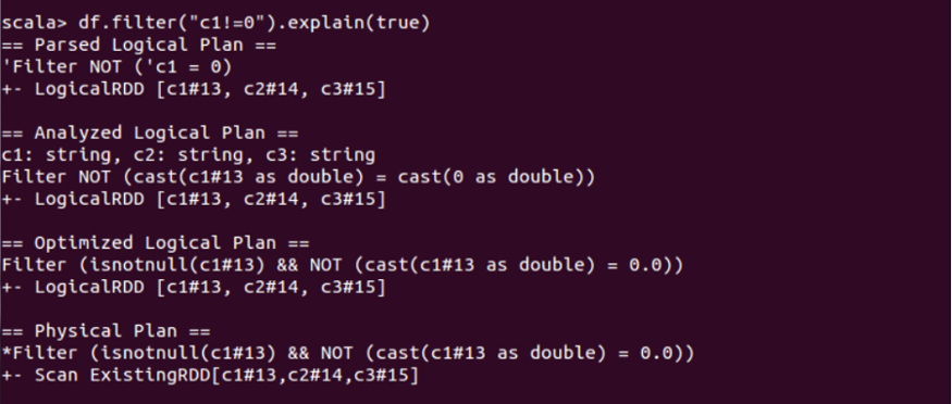 explain function with the true argument
It is crystal clear from the above image that all plans look the same. Now, in order to differentiate between the optimized logical plan and the analyzed logical plan, we should run this example with two filters:
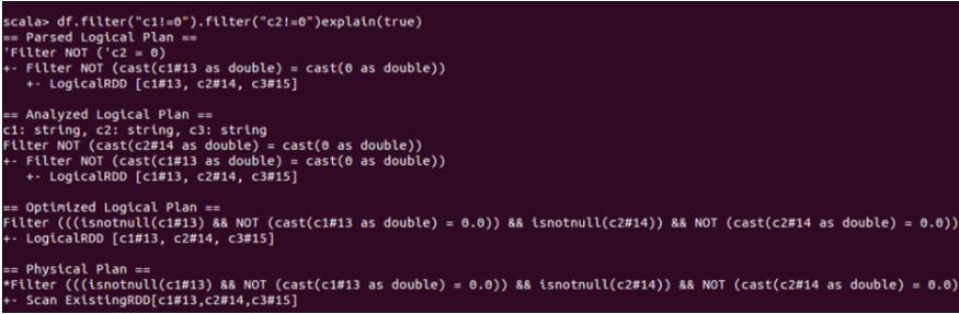 explain function with true argument and multiple filters
Here is the actual difference:
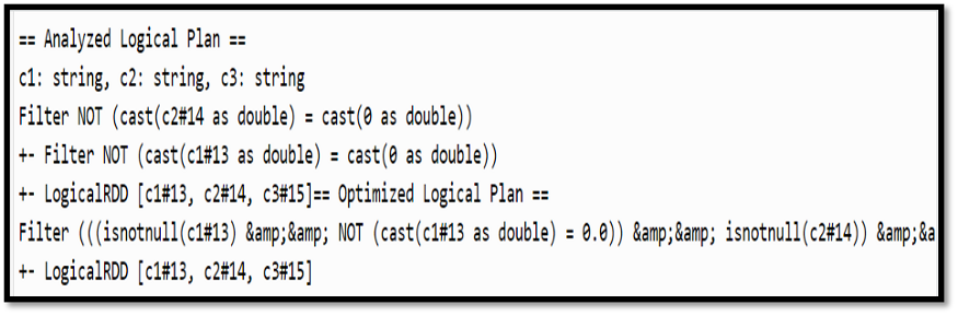 Analyzed Logical Plan
Spark performs optimization by itself in the optimized logical plan. It can figure out that there is no requirement for two filters. Instead, it completes execution in one filter because the same task can be done by using just one filter through the ‘and’ operator.
First part: Unresolved/Parsed Logical plan generation
-
The first step contributes to the generation of an Unresolved Logical Plan.
-
We call it an Unresolved Logical Plan because the column or table names may be inaccurate or even exist even when we have a valid code and correct syntax. So, it can be concluded that Spark creates a blank Logical Plan at this step where there are no checks for the column name, table name, etc.
-
This plan is generated post verifying that everything is correct on the syntactic field. Next, the first version of a logical plan is produced where the relation name and columns are not specifically resolved after the semantic analysis is executed. This produces a result as provided below:
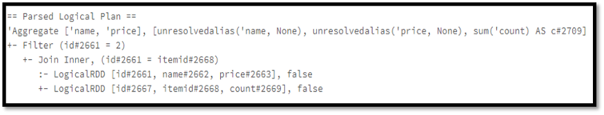 Spark Unresolved/Parsed Logical plan
Second part: Resolved/Analyzed Logical plan generation
-
After the generation of an unresolved plan, it will resolve everything unresolved yet by accessing an internal Spark structure mentioned as “Catalog” in the previous schema.
-
“Catalog” is a repository of Spark table, DataFrame, and DataSet. The data from meta-store is pulled into an internal storage component of Spark (also know as Catalog).
-
“Analyzer” helps us to resolve/verify the semantics, column name, table name by cross-checking with the Catalog. DataFrame/DataSet starts performing analysis without action at the time of creating the Logical Plan. That’s why DataFrame/DataSet follows a Semi-lazy evaluation. Let’s take an example: dataFrame.select(“price”) //Column “price” may not even exist.
-
The analyzer can reject the Unresolved Logical Plan when it is not able to resolve them (column name, table name, etc.). It creates a Resolved Logical Plan if it is able to resolve them.
-
Upon successful completion of everything, the plan is marked as “Analyzed Logical Plan” and will be formatted as shown below:
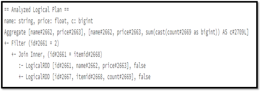 Spark Resolved/Analyzed Logical plan
Third part: Optimized logical Plan
-
In order to resolve the Analyzed logical plans, they are sent through a series of rules. The optimized logical plan is produced as a result. Spark is normally allowed to plug in a set of optimization rules by the optimized logical plan.
-
The Resolved Logical plan will be passed on to a “Catalyst Optimizer” after it is generated. Catalyst Optimizer will try to optimize the plan after applying its own rule. Basically, the Catalyst Optimizer is responsible to perform logical optimization. For example,
1) It checks all the tasks which can be performed and computed together in one Stage.
2) It decides the order of execution of queries for better performance in the case of a multi-join query.
3) It tries to optimize the query by evaluating the filter clause before any project.
-
Optimized Logical Plan is generated as a result.
-
In case of a specific business use case, it is possible to create our own customized Catalyst Optimizer to perform custom optimization after specific rules are defined/applied to it.
When the optimization ends, it will produce the below output:
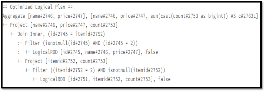 Spark optimized logical plan
What is a Spark Physical Plan?
Physical Plan is an internal enhancement or optimization for Spark. It is generated after creation of the Optimized Logical Plan .
What exactly does Physical Plan do?
-
Suppose, there’s a join query between two tables. In that join operation, one of them is a large table and the other one is a small table with a different number of partitions scattered in different nodes across the cluster (it can be in a single rack or a different rack). Spark decides which partitions should be joined at the start (order of joining), the type of join, etc. for better optimization.
-
Physical Plan is limited to Spark operation and for this, it will do an evaluation of multiple physical plans and finalize the suitable optimal physical plan. And ultimately, the finest Physical Plan runs.
-
Once the finest Physical Plan is selected, executable code (DAG of RDDs) for the query is created which needs to be executed in a distributed manner on the cluster.
-
This entire process is known as Codegen and that is the task of Spark’s Tungsten Execution Engine.
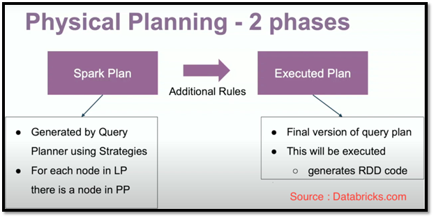 Physical Planning Phases
Physical plan is:
-
A bridge between Logical Plans and RDDs
-
It is a tree
-
Contains more specific description of how things (execution) should happen (specific choice of algorithm)
-
User lower-level primitives (RDDs)
Example :
Y = product.join(prod_orders,product.id=prod_orders.itemid,’inner’)
.where(col(“product.id”) ==2)
.groupBy(“name”, “price”).agg(sum(“count”))
.alias(“C”)
Or
X = spark.sql(“select product.name,product.price,sum(prod_orders.count) as
c, from product, prod_orders where product.id=prod_orders.itemid and
product.id=2 group by product.name,product.price”)
Y.explain();
X.explain();
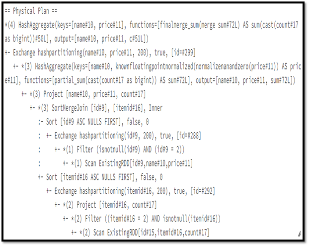 Spark Physical Plan
-
explain(mode=”simple”) shows physical plan.
-
explain(mode=”extended”) presents physical and logical plans.
-
explain(mode=”codegen”) shows the java code planned to be executed.
-
explain(mode=”cost”) presents the optimized logical plan and related statistics (if they exist).
-
explain(mode=”formatted”) shows a split output created by an optimized physical plan outline, and a section of every node detail.
Conclusion
-
Logical Plan simply illustrates the expected output after a series of multiple transformations like join, groupBy, where, filter, etc. clauses are applied on a particular table.
-
Physical Plan is accountable for finalizing the join type, the sequence of the execution of operations like filter, where, groupBy clause, etc.
Learn Watermarking in Spark Structured Streaming with our blog here. To get the best data engineering solutions for your business, reach out to us at Clairvoyant.
References:
https://databricks.com/session_eu19/physical-plans-in-spark-sql
https://medium.com/datalex/sparks-logical-and-physical-plans-when-why-how-and-beyond-8cd1947b605a