During the pandemic, more and more people are getting access to the internet. This has certainly increased the rise in web traffic for almost every website. Web traffic can be defined as the number of requests sent and received by users to a website; it has been the largest portion of Internet traffic. Predicting this web traffic will help us to avoid website crashes and downtime and to be prepared by using certain measures like load balancing for the web traffic and in turn, provide a better user experience for every user of the website. The goal is to predict future web traffic to make better traffic control decisions. For this, we will be needing time series forecasting. Time series forecasting has been a hot topic for all researchers.
Importance of Time Series:
Time series is statistical data arranged and presented in a chronological order which is spread over a period of time. Time series analysis and forecasting are among the most common quantitative techniques that are used by businesses and researchers today. Some examples of time series databases are financial market database, weather forecasting database, smart home monitoring database, supply chain monitoring databases, and many more.
The most widely used models for time series analysis are:
-
Holt Winters Algorithm
-
AR Models
-
MA Models
The above models are used for linear prediction for time series analysis. For non-linear predictions, we have recurring neural network models.
In this blog post, we will be using ARIMA models and LSTM models for predictions.
Dataset:
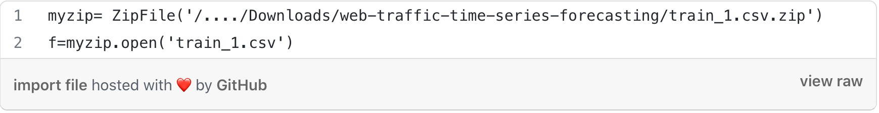
The dataset that we used in this blog post can be downloaded from here.
It is a competition held by Google for time series prediction for web trafficking.
The dataset contains the following information:
-
Train.csv- Contains 145k rows each of which represents a different Wikipedia page and it has 551 columns.
-
Key.csv- Has the number of rows equal to the number of predictions we have to make. There are two columns in this file- ‘page name’ and ‘id’.
There are two approaches that are being used for the prediction. They are as follows:
-
ARIMA MODEL
-
LSTM MODEL
ARIMA Model:
ARIMA stands for AutoRegressive Integrated Moving Average. It is a class of statistical models for analyzing and forecasting time series data.
A quick breakdown of the components of the ARIMA model:
AR- AutoRegression: Model that uses the dependent relationship between an observation and some number of lagged observations.
I- Integrated: The use of differencing of raw observations in order to make the time series stationary.
MA- Moving Average: A model that uses the dependency between an observation and a residual error from a moving average model applied to lagged observations.
ARIMA models describe the trends and seasonality in time series as a function of lagged values and Averages changing over time intervals.
The parameters of the ARIMA model are as follows:
-
p - The number of lag observations included in the model, also called the lag order.
-
d - The number of times that the raw observations are different, also called the degree of differencing.
-
q - The size of the moving average window, also called the order of moving average.
For further information please visit here.
LSTM Model:
Long Short Term Memory is a type of recurrent neural network capable of learning order dependence in sequence prediction problems.
LSTMs are explicitly designed to avoid the long-term dependency problem. Remembering information for long periods of time is practically the default behavior. In standard RNNs, this repeating module will have a very simple structure, such as a single tanh layer.
-2.png)
LSTMs also have this chain-like structure, but the repeating module has a different structure. Instead of having a single neural network layer, there are four, interacting in a very special way.
-1.png)
For further information please visit this link.
Now moving to address the problem:
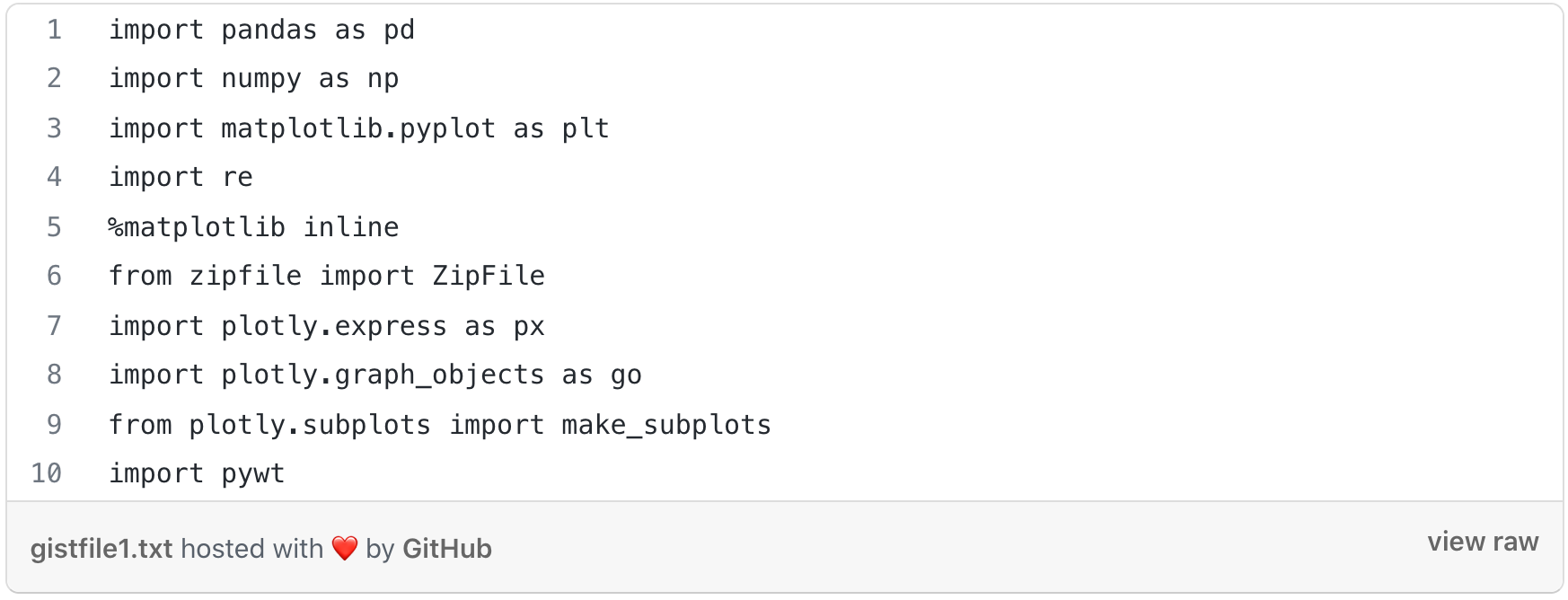
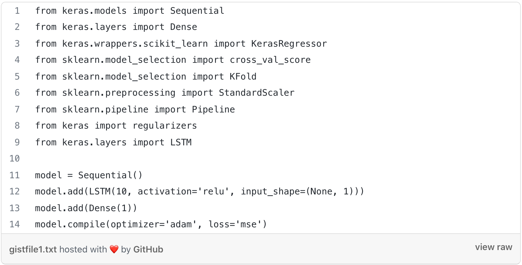
1. Importing the libraries:
2. Reading the CSV file:

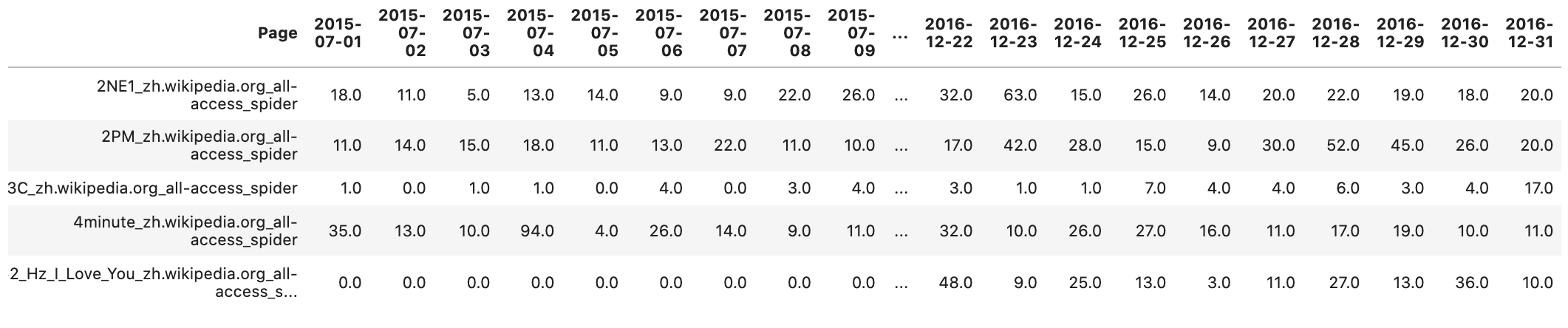
3. We have more than 145k time series, and analyzing them is impossible. So we are going to combine different types of pages and then analyze them together.
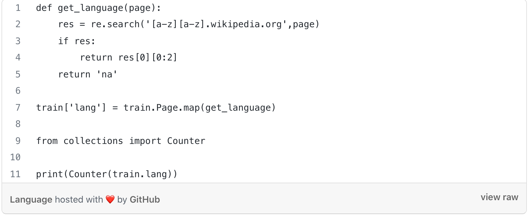
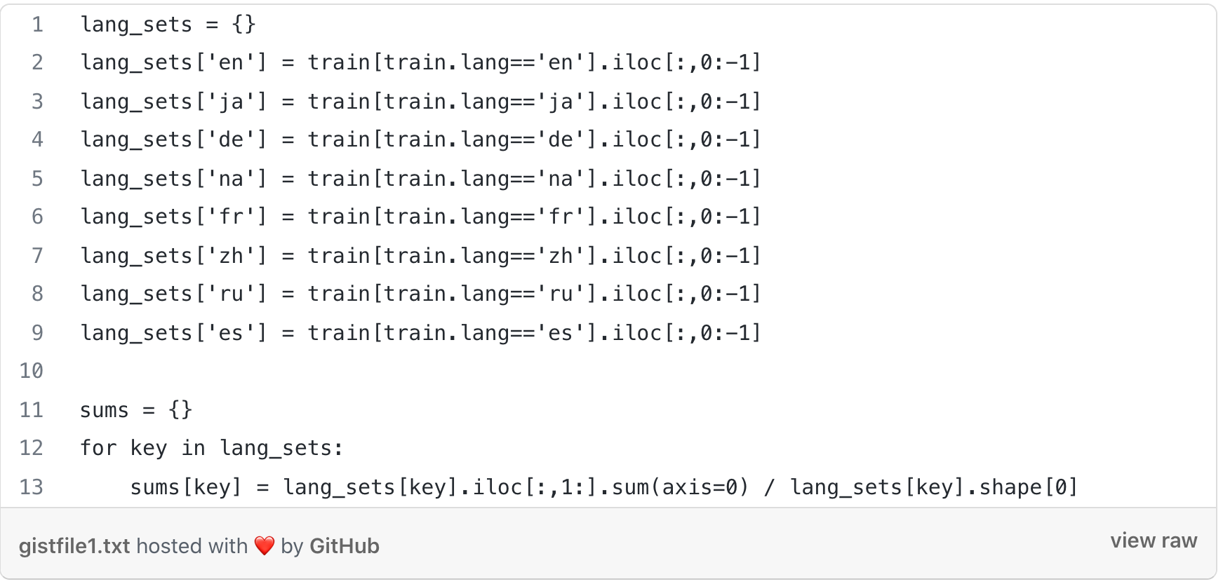
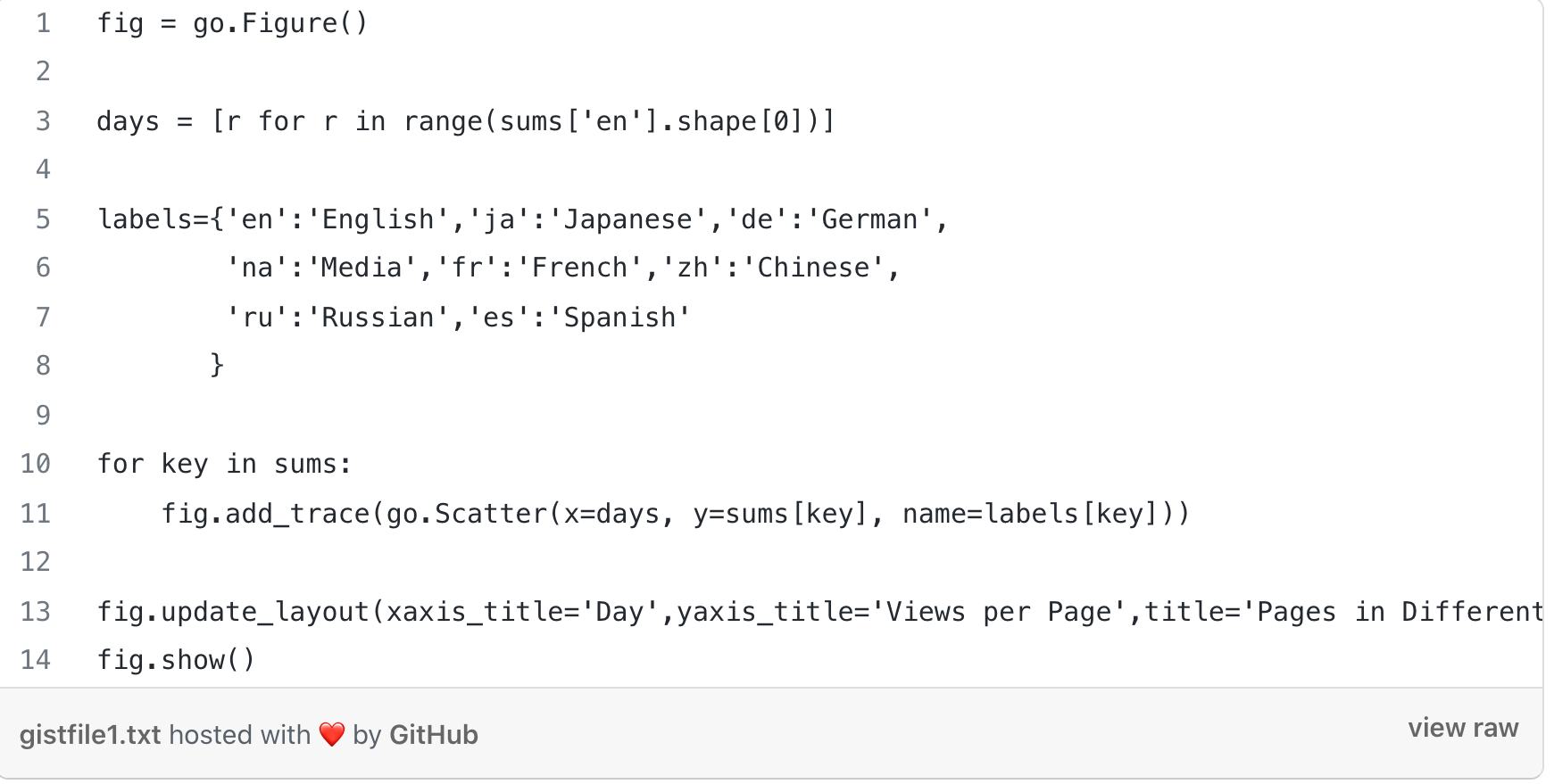
The letters correspond to different languages:
en- English, ja- Japanese, de- German, fr- French, zh- Chinese, ru- Russian, es- Spanish.
-2.png)
4. Building Model:
-
ARIMA Model:
ARIMA models describe the trends and seasonality in time series as a function of lagged values and Averages changing over time intervals. The model includes Differencing time series (forming a new time series by subtracting the previous observation from the current time).
The ARIMA model has two important components:
-
Auto-Regressive (AR) part.
-
Moving Average (MA) part.
Splitting the data into training and test set:
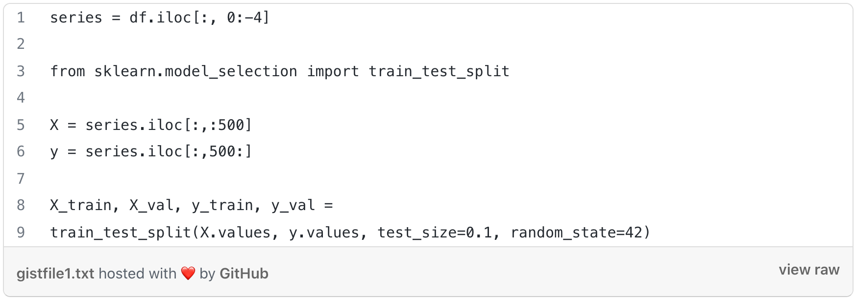
Now, we will be using the Walk Forward Validation technique to see how the ARIMA Model is learning and then predicting. There are two ways to split time series into training and validation datasets:
-
Walk-forward split: This is not actually a split - we train on the complete dataset and validate on the complete dataset, using different timeframes. Timeframe for validation is shifted forward by one prediction interval relative to the time frame for training.
-
Side-by-side split: This is a traditional split model for mainstream machine learning. Dataset is split into independent parts, one part used strictly for training and another part used strictly for validation.
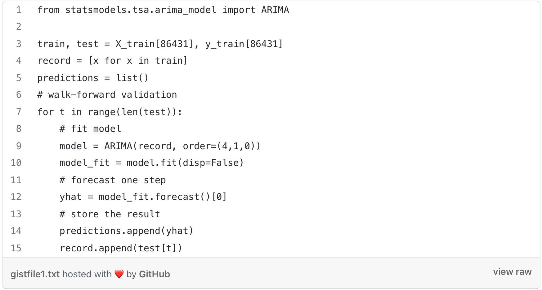
For our model, ARIMA(4,1,0) means that we are describing some response variable (Y) by combining a 4th order Auto-Regressive model and a 0th order Moving Average model. A good way to think about it is (AR, I, MA). This makes our model look the following, in simple terms: Y = (Auto-Regressive Parameters) + (Moving Average Parameters) The 1 in between 4 and 0 represents the 'I' part of the model (the Integrative part), and it signifies a model where we’re taking the difference between response variable data.
The ARIMA Model gives better results with a smaller dataset. So we implemented this on a smaller dataset to see how the predictions were.
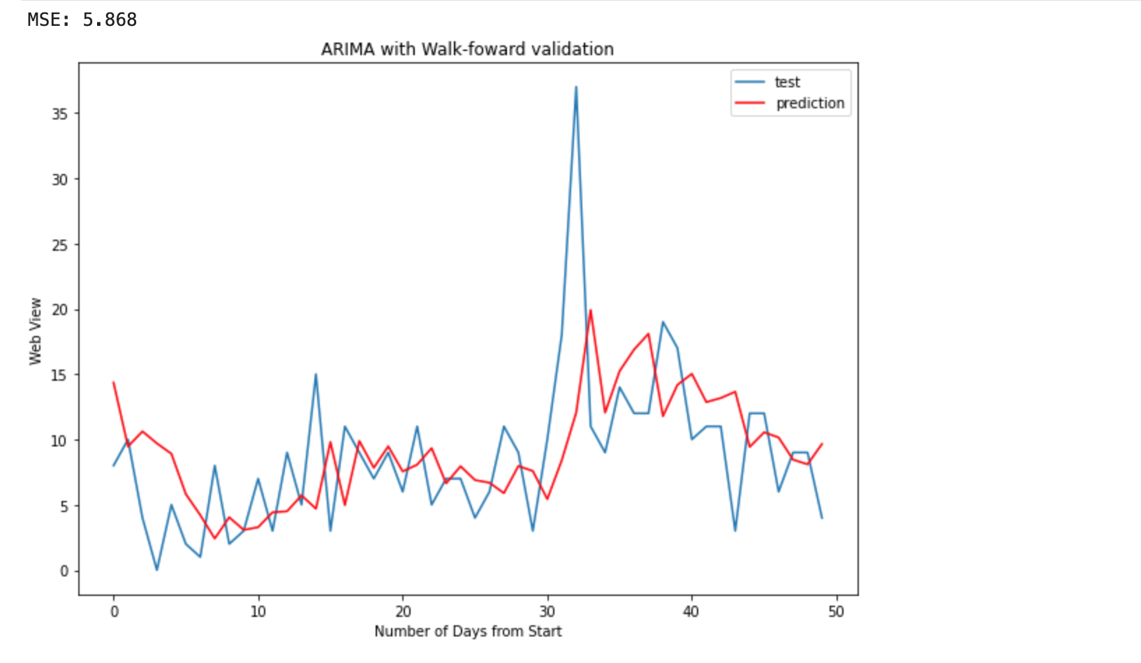
The above graph gives us the idea that a lot of prediction points were not meeting their true value.
For evaluation, we used the RMSE. The RMSE obtained was 5.868.
-
LSTM Model:
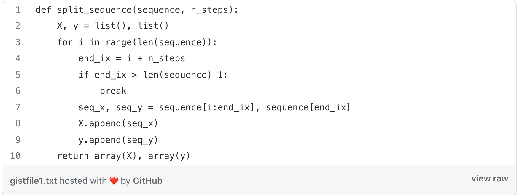
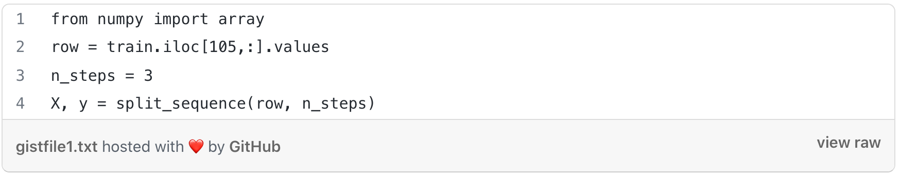
For this model, we first split the data into X and y, find the end of the pattern, and then gathered the input and output of the pattern.
We split the dataset into a test and train set by taking the first 70% as the training set and the remaining 30% as a test set.

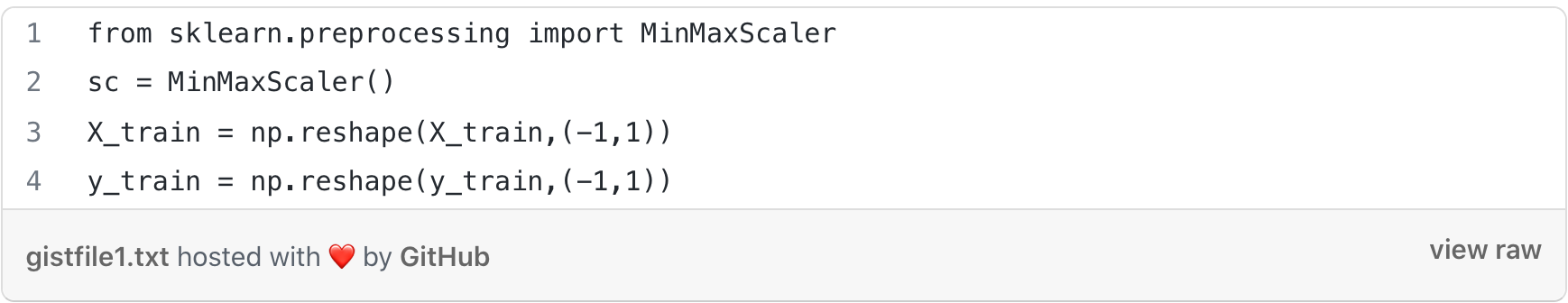
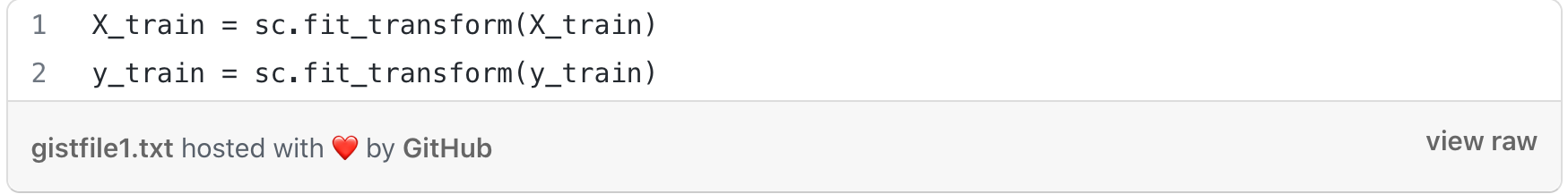
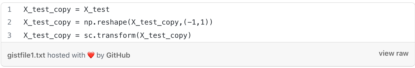
To normalize the dataset we used MinMaxScaler to rescale our dataset. First, a MinMaxScaler instance was defined with default hyperparameters. Once defined, we called the fit_transform() function and passed it to our dataset to create a transformed version of our dataset.
Training the model with LSTM:
The output layer consisted of a Dense layer with 1 neuron with activation as ReLU.
The optimizer used for training the model was Adam optimizer and the loss was calculated through MSE.
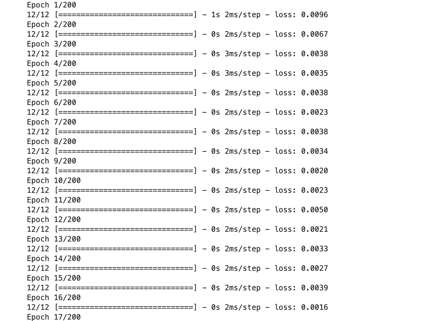
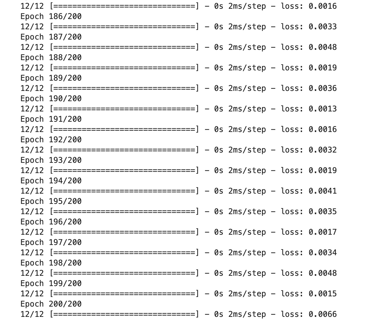
We trained the model with 200 epochs.
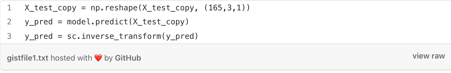
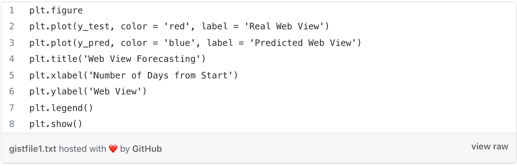
Plotting the graph:
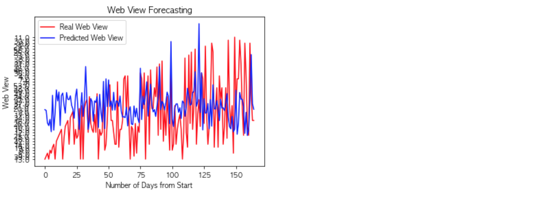
This LSTM model contains only a single hidden LSTM layer. We used Relu as an activation function and 10 neurons in the LSTM layer. The MSE we finally reached was 0.0066.
Conclusion
Web traffic time series predictions can be done easily by ARIMA and LSTM, but predicting time series itself is a hard problem. By looking at the graph we can say that whenever there is an occasional trend, there has been a spike in the views of the website and it has affected the overall model performance. The occasional trends in the model are considered outliers. To improve the model we can first exclude the outliers in the data and then train the model.
For future work, we can combine the results of the LSTM and the ARIMA model and then see how the model gives the prediction. This can be done for future experiments. I hope you found the blog post informative and enjoyed it.
Check out our artificial intelligence services for all your business requirements.
References
https://medium.com/swlh/wikipedia-web-traffic-time-series-forecasting-part-1-e43734adca3d
https://medium.com/@jyshao53/web-traffic-time-series-prediction-using-arima-lstm-7ef3911845ae
https://www.kaggle.com/arjunsurendran/using-lstm-on-training-data