Example of Deep Learning to analyze audio signals to determine the music Genre Convolutional Neural Networks
“If Music is a Place — then Jazz is the City, Folk is the Wilderness, Rock is the Road, Classical is a Temple.” — Vera Nazarin
We’ve all used some music streaming app to listen to music. But what is the app's logic for creating a personalized playlist for us?
One general example of logic is by having a Music Genre Classification System.
Music genre classification forms a basic step for building a strong recommendation system.
The idea behind this project is to see how to handle sound files in python, compute sound and audio features from them, run Machine Learning Algorithms on them, and see the results.
In a more systematic way, the main aim is to create a machine learning model, which classifies music samples into different genres. It aims to predict the genre using an audio signal as its input.
The objective of automating the music classification is to make the selection of songs quick and less cumbersome. If one has to manually classify the songs or music, one has to listen to a whole lot of songs and then select the genre. This is not only time-consuming but also difficult. Automating music classification can help to find valuable data such as trends, popular genres, and artists easily. Determining music genres is the very first step towards this direction.
Dataset
For this project, the dataset that we will be working with is GTZAN Genre Classification dataset which consists of 1,000 audio tracks, each 30 seconds long. It contains 10 genres, each represented by 100 tracks.
The 10 genres are as follows:
-
Blues
-
Classical
-
Country
-
Disco
-
Hip-hop
-
Jazz
-
Metal
-
Pop
-
Reggae
-
Rock
The dataset has the following folders:
-
Genres original — A collection of 10 genres with 100 audio files each, all having a length of 30 seconds (the famous GTZAN dataset, the MNIST of sounds)
-
Images original — A visual representation for each audio file. One way to classify data is through neural networks because NN’s usually take in some sort of image representation.
-
2 CSV files — Containing features of the audio files. One file has for each song (30 seconds long) a mean and variance computed over multiple features that can be extracted from an audio file. The other file has the same structure, but the songs are split before into 3 seconds audio files.
Let’s now dive into the code part of the project…
Reading and Understanding the Data
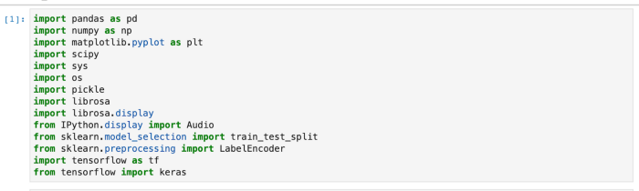
1. Importing Libraries
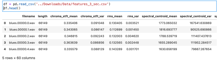
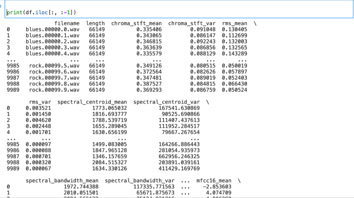
2. Read the CSV file
3. About the Dataset

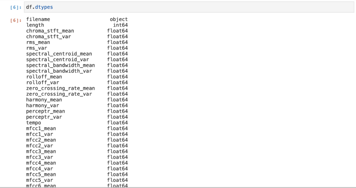
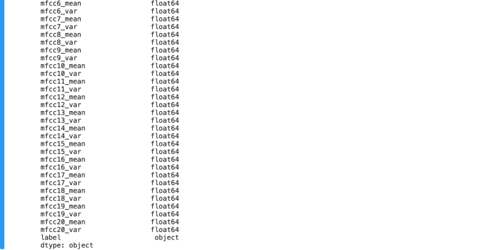
This returns the Data Types in the Dataframe. It is used to help us understand what data we’re dealing with in the dataset.
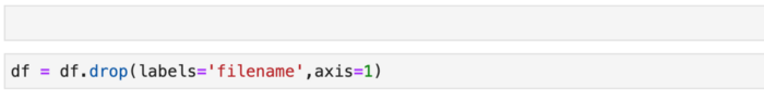
First, we’ll drop the first column ‘filename’ as it is unnecessary:
Understanding the Audio Files
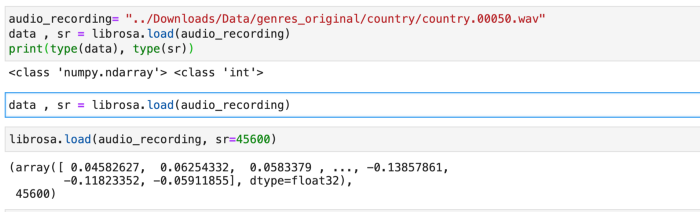
Through this code:
data, sr = librosa.load(audio_recording)
It loads and decodes the audio as a time series y.
sr = sampling rate of y. It is the number of samples per second. 20 kHz is the audible range for human beings. So it is used as the default value for sr. In this code we are using sr as 45600Hz.
Audio Libraries Used
1. LIBROSA
Librosa is a python package for music and audio analysis. It provides the building blocks necessary to create music information retrieval systems. By using Librosa, we can extract certain key features from the audio samples such as Tempo, Chroma Energy Normalized, Mel-Freqency Cepstral Coefficients, Spectral Centroid, Spectral Contrast, Spectral Rolloff, and Zero Crossing Rate. For further information on this, please visit here.
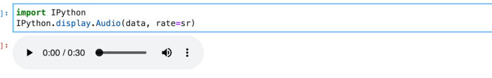
2. Python.display.Audio
With the help of IPython.display.Audio we can play audio in the notebook. It is a library used for playing the audio in the jupyterlab. The code is below:
Visualizing Audio Files
The following methods are used for visualizing the audio files we have:
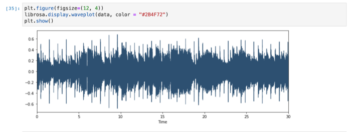
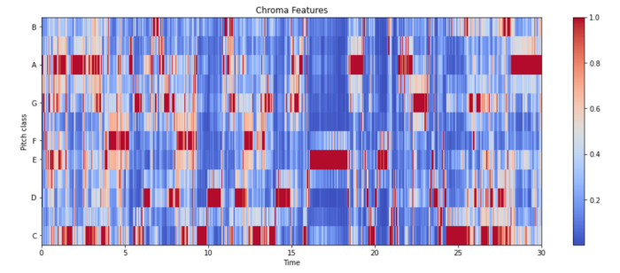
1. Plot Raw Wave Files
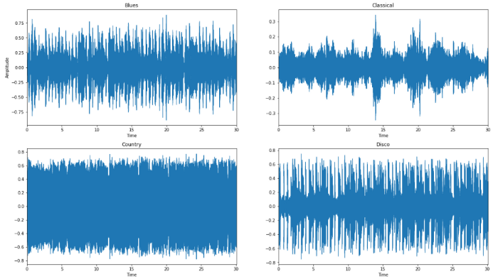
Waveforms are visual representations of sound as time on the x-axis and amplitude on the y-axis. They are great for allowing us to quickly scan the audio data and visually compare and contrast which genres might be more similar than others. For deeper knowledge on this please visit here.
2. Spectrograms
A spectrogram is a visual way of representing the signal loudness of a signal over time at various frequencies present in a particular waveform. Not only can one see whether there is more or less energy at, for example, 2 Hz vs 10 Hz, but one can also see how energy levels vary over time.
Spectrograms are sometimes called sonographs, voiceprints, or voicegrams. When the data is represented in a 3D plot, they may be called waterfalls. In 2-dimensional arrays, the first axis is frequency while the second axis is time.
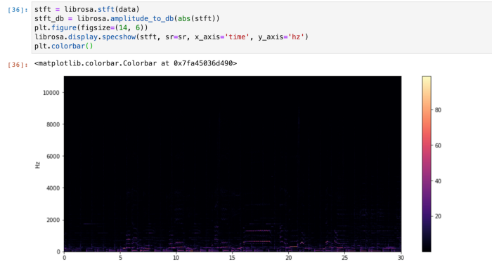
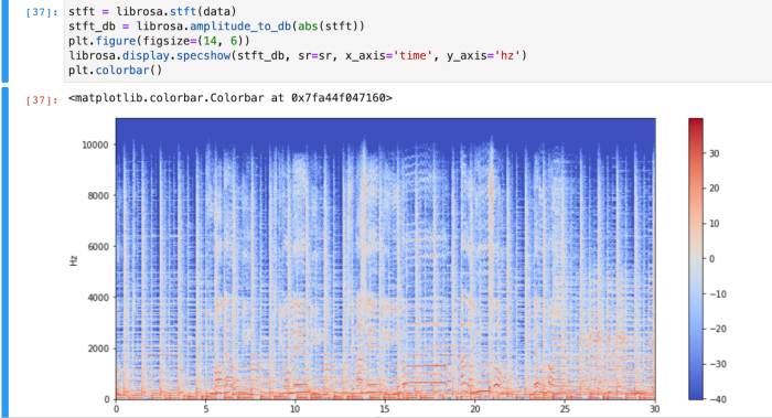
The vertical axis represents frequencies (from 0 to 10kHz), and the horizontal axis represents the time of the clip.
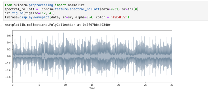
3. Spectral Rolloff
Spectral Rolloff is the frequency below which a specified percentage of the total spectral energy, e.g. 85%, lies
librosa.feature.spectral_rolloff computes the rolloff frequency for each frame in a signal.
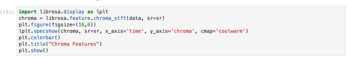
4. Chroma Feature
It is a powerful tool for analyzing music features whose pitches can be meaningfully categorized and whose tuning approximates to the equal-tempered scale. One main property of chroma features is that they capture harmonic and melodic characteristics of music while being robust to changes in timbre and instrumentation. For more information visit here.
5. Zero Crossing Rate
Zero crossing is said to occur if successive samples have different algebraic signs. The rate at which zero-crossings occur is a simple measure of the frequency content of a signal. Zero-crossing rate is a measure of the number of times in a given time interval/frame that the amplitude of the speech signals passes through a value of zero.
Through the librosa library, we can get the count of zero crossings in the audio:

Feature Extraction
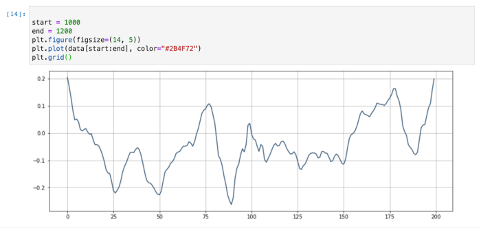
Preprocessing of data is required before we finally train the data. We will try and focus on the last column that is ‘label’ and will encode it with the function LabelEncoder() of sklearn.preprocessing.
We can’t have text in our data if we’re going to run any kind of model on it. So before we can run a model, we need to make this data ready for the model. To convert this kind of categorical text data into model-understandable numerical data, we use the Label Encoder class. For further information visit here.

fit_transform(): Fit label encoder and return encoded labels.
Scaling the Features
Standard scaler is used to standardize features by removing the mean and scaling to unit variance.
The standard score of sample x is calculated as:
z = (x - u) / s
Standardization of a dataset is a common requirement for many machine learning estimators: they might behave badly if the individual features do not more or less look like standard normally distributed data.

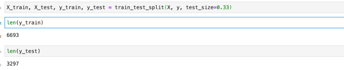
Dividing Data Into Training and Testing Sets
Building the Model
Now comes the last part of the music classification genre project. The features have been extracted from the raw data and now we have to train the model. There are many ways through which we can train our model. Some of these approaches are:
-
Multiclass Support Vector Machines
-
K-Means Clustering
-
K-Nearest Neighbors
-
Convolutional Neural Networks
For this blog, we will be using CNN Algorithm for training our model. We chose this approach because various forms of research show it to have the best results for this problem.
The following chart gives a clear view of why CNN algorithm is used:
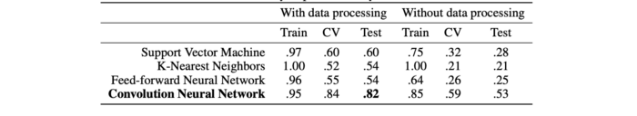
For further information please visit this site.
Model Evaluation
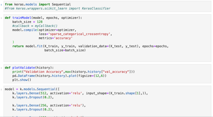
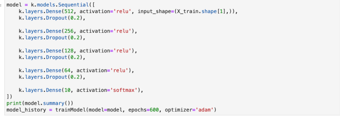
For the CNN model, we had used the Adam optimizer for training the model. The epoch that was chosen for the training model is 600.
All of the hidden layers are using the RELU activation function and the output layer uses the softmax function. The loss is calculated using the sparse_categorical_crossentropy function.
Dropout is used to prevent overfitting.
We chose the Adam optimizer because it gave us the best results after evaluating other optimizers.
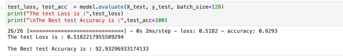
The model accuracy can be increased by further increasing the epochs but after a certain period, we may achieve a threshold, so the value should be determined accordingly.
The accuracy we achieved for the test set is 92.93 percent which is very decent.
So we come to the conclusion that Neural Networks are very effective in machine learning models. Tensorflow is very useful in implementing Convolutional Neural Network (CNN) that helps in the classifying process. Also, learn about image caption generator in our blog here.
Hope you enjoyed the post and found it informative. To get the best artificial intelligence solutions for your business, reach out to us at Clairvoyant.
References
https://towardsdatascience.com/extract-features-of-music-75a3f9bc265d
https://towardsdatascience.com/music-genre-classification-with-python-c714d032f0d8