Survival Analysis is a branch of statistics that helps modeling the time that might take for a particular event to occur¹. Hence, it is often called ‘time-to-event’ analysis. This was majorly used in medical and biological disciplines to study the survival times of patients suffering from major diseases like cancer, organ failure, etc. Gradually, its usage picked up in other fields like economics, machine maintenance, marketing, insurance, etc. Survival curves has always played a key role in Actuarial Sciences to outline the incidence of the demise of a person at different ages given certain health conditions. Based on the probabilities of survival of policyholders, actuaries fix an appropriate insurance premium.
Key terms of survival analysis
The following terms are commonly used in survival analysis:
· Event²: Occurrence of death, disease, disease recurrence, recovery from illness, customer churn, etc.
· Time line: The time from the beginning of an observation period to its end (like from the time a customer signs the contract till churn or end of the study)
· Time of event Occurrence (T): Random time at which the event may occur
· Censoring / Censored observations²: Subjects who haven’t encountered an event during the observation time are described as censored. A censored subject may or may not have an event after the end of observation time. An example is a customer who hasn’t yet churned at the time of the study. Such observations are said to be right-censored
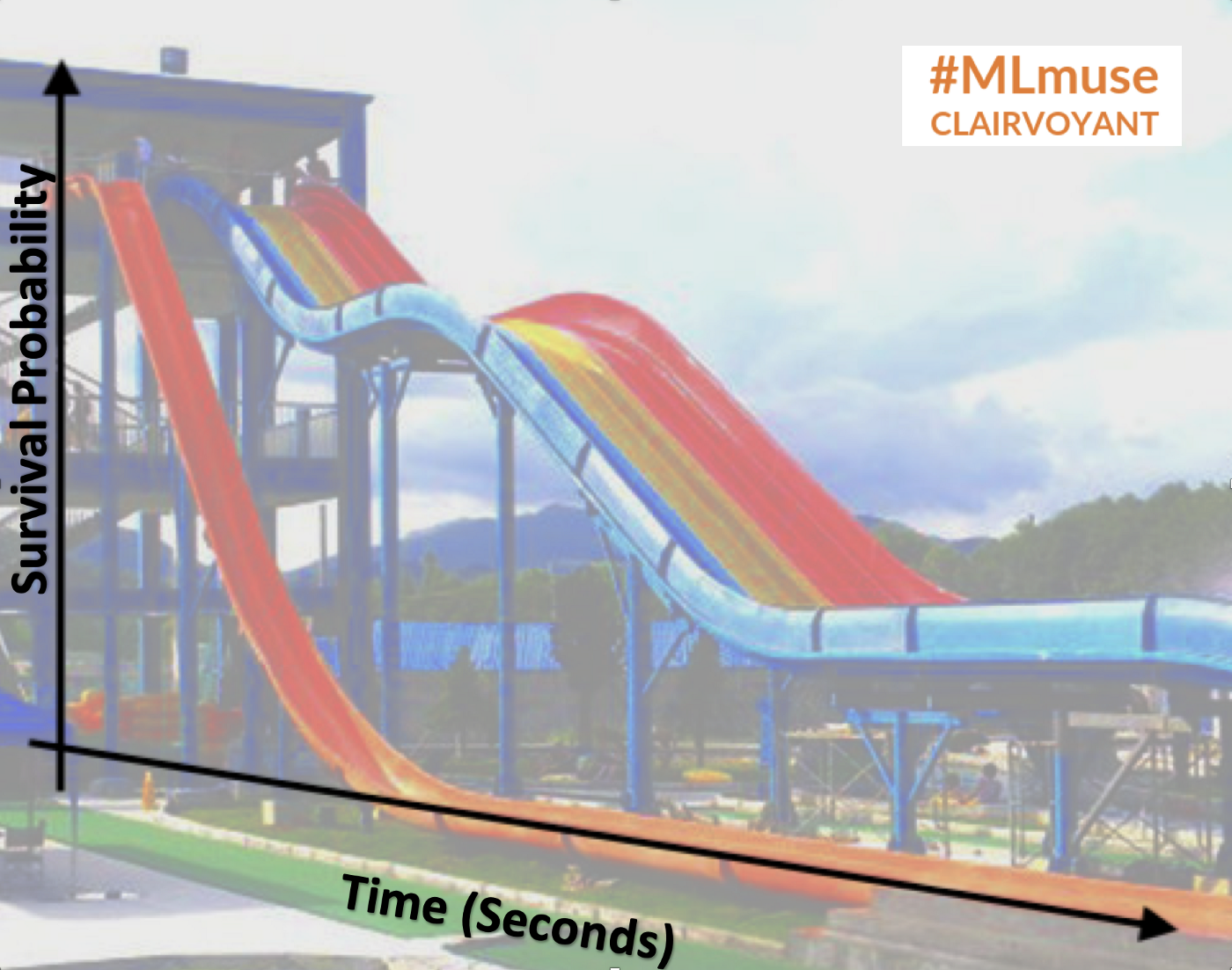
· Survival function, S(t): It is the probability that a subject survives longer than a certain time ‘t’ which means,
S(t) = Probability(T > t)
Generally, S(0) = 1 for example, at t = 0 i.e., when a contract has just begun, 100% of the customers will stay in the contract beyond t = 0.
When and where to use?
Survival analysis can be applied,
- In scenarios where time-to-event information can be more beneficial than the information on whether or not an event may occur
- Presence of censored events: It is common in most cases to have subjects who did not experience an event by the end of a study
In problems like:
- What can be the expected lifetime of patients who have undergone a heart transplant?
- How long it might take for a customer to churn
- After how many days might a patient get readmitted after a major medical procedure?
o How long can we expect a user to be on a website?
and many more situations.
Why not logistic/ linear regression models?
Outcomes of a problem come in varied statistical forms:
-
If an outcome is continuous, we can easily use linear regression. If an outcome is discrete like ‘either-or’, logistic regression can be used. However, if the time for an event to occur is the observed outcome, survival analysis can be one of the techniques to model the outcome
-
The outcome of survival analysis is ‘time’ which is strictly positive and this outcome need not be normally distributed whereas linear regression requires that the target variable be normally distributed
-
Logistic regression can only tell us if a customer will churn or not churn. If a customer is predicted not to churn, it doesn’t imply that the customer will never churn. If not now, there are good chances that a customer might churn after a certain period of time. In such cases, survival analysis can throw light on such censored customers by determining the probability of survival of a customer after various points of time
Estimating Survival Function using Kaplan-Meier (KM) estimate
In real scenarios, we do not usually have the actual survival function of a population. Hence, survival function is usually estimated from the observed data using Kaplan-Meier (KM) curve with time (duration of an observation- least to the last) on its x-axis and the probability of survival or proportion of subjects surviving on the y-axis. A vertical drop in the curve denotes the occurrence of the event.
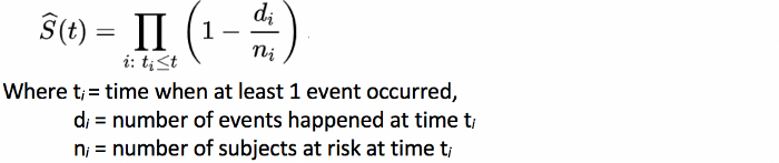
KM estimator(or product limit estimator) is a non-parametric statistic named after Edward L. Kaplan and Paul Meier, used to estimate the survival function at time t, given by:
Survival Curves use-case in customer churn analysis:
The Python package for survival analysis is ‘lifelines’ or even scikit-survival analysis and R package is ‘survival’.
Let’s consider a subset of customer churn data of a Malaysian telecom operator:
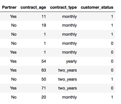
At any given time, predicting how long the customer will stay active (i.e not churn) will be more informative than just predicting whether or not a customer will churn at a given time. For this data, customer_status = 0 is not_churn, 1 is churn.
Here, birth event → customer joining, death event → customer churn, censorship → is the current time, doesn’t allow us from seeing all customer cancelations/churns.
So we have,
Event → ‘Customer_status = 1’ which means the customer is inactive, which in turn means that the customer churn occurred
Time line → ‘contract_age’ starting and ending times of contract duration observed
Censor → At the time (t), if customer_status = 0 implies that ‘Churn’ has not been observed for those customers (as non-occurrence of an event is called censored)
So now, knowing a survival curve completely defines the population’s distribution of lifetimes, like what could be the maximum time until a customer can stay active
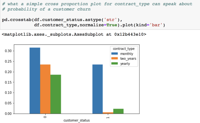
This proportion plot can tell us that the maximum proportion of ‘Churns’ are among the customers whose contract_type = monthly.
Let’s now see what other information we can gather using survival curves…
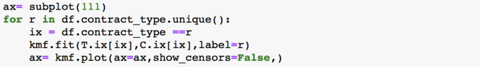
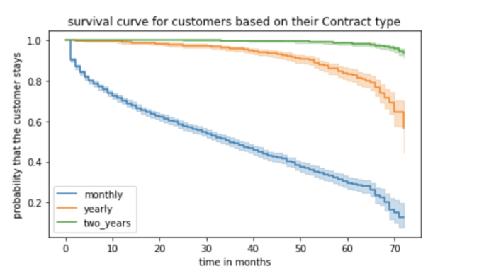
These are the survival curves for customers based on the predictor, ‘contract_type’. As we can notice:
- The probability of survival is the highest among customers whose contract period is two years. We can say with more than 98% probability that these customers will stay active (not churn) even after 50 months
- For yearly contract customers, the probability of survival starts dropping after 50 months (after 4 years). It indicates a need to introduce some customer retention interventions to prevent their churn
-For monthly contract customers, there’s a significant drop immediately after a couple of months
Conclusion:
Survival curves can be very informative compared to a proportion plot. KM curves can also be used for comparison like the one above shows a significant difference in survival probabilities of customers of different contract types. KM estimates are best suited when a predictor variable is categorical (like contract_type).
In the next article, we will be using Cox’s proportional hazard regression methods for a continuous predictor and for investigating the effect of several variables upon time to event. We will also see how survival curves can be used to predict a new customer’s lifeline. Also check out our blog "Cox Proportional Hazards Model for Survival Analysis: #MLmuse", here. To get the best artificial intelligence solutions for your business, reach out to us at Clairvoyant.
References:
¹Julia Kagan., (May, 2018): Survival Analysis. Retrieved from-
https://www.investopedia.com/terms/s/survival-analysis.asp
²Survival Analysis. Retrieved from-
https://en.wikipedia.org/wiki/Survival_analysis